Research · Publication & note
Pump-and-probe optical transmission phase shift as a quantitative probe of the Bogoliubov dispersion relation in a nonlinear channel waveguide - Notes
Research article
Published abstract
We theoretically investigate the dispersion relation of small-amplitude optical waves superimposing upon a beam of polarized monochromatic light propagating along a single-mode channel waveguide characterized by an instantaneous and spatially local Kerr nonlinearity. These small luminous fluctuations propagate along the waveguide as Bogoliubov elementary excitations on top of a one-dimensional dilute Bose quantum fluid evolve in time. They consequently display a strongly renormalized dispersion law, of Bogoliubov type. Analytical and numerical results are found in both the absence and the presence of one- and two-photon losses. Silicon and silicon-nitride waveguides are used as examples. We finally propose an experiment to measure this Bogoliubov dispersion relation, based on a stimulated four-wave mixing and interference spectroscopy techniques.
Figures
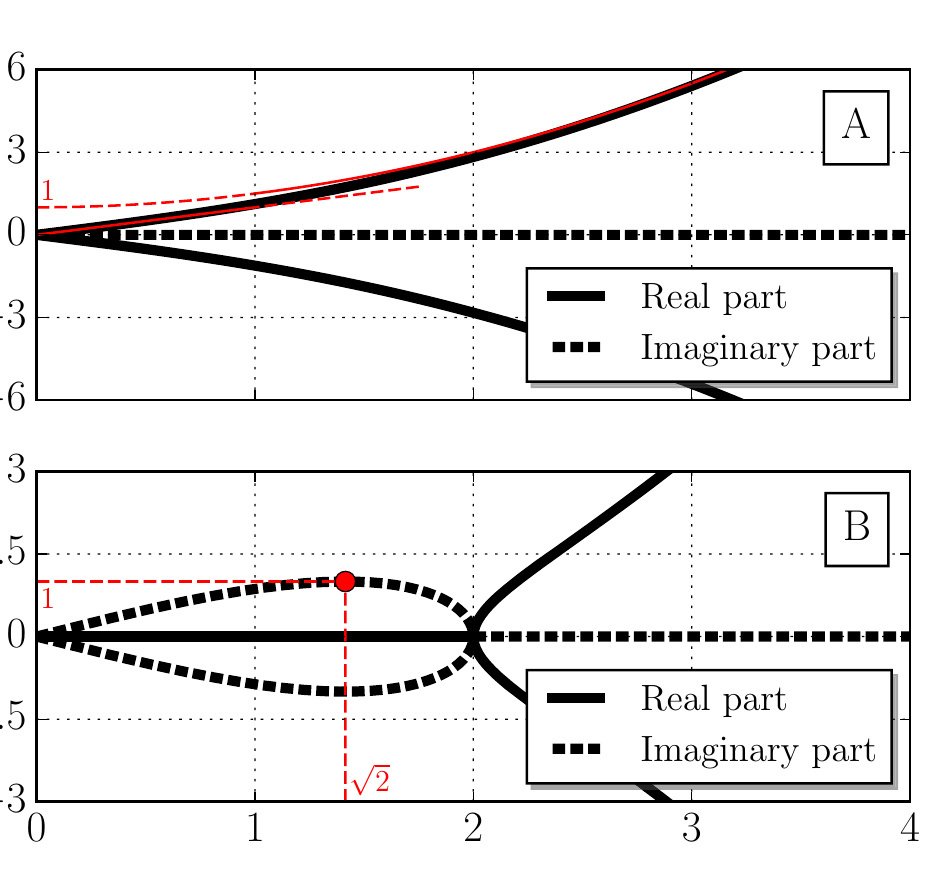
Source: P.-É. Larré et al., European Physical Journal D 71, 146 (2017). © EDP Sciences, SIF and Springer-Verlag.
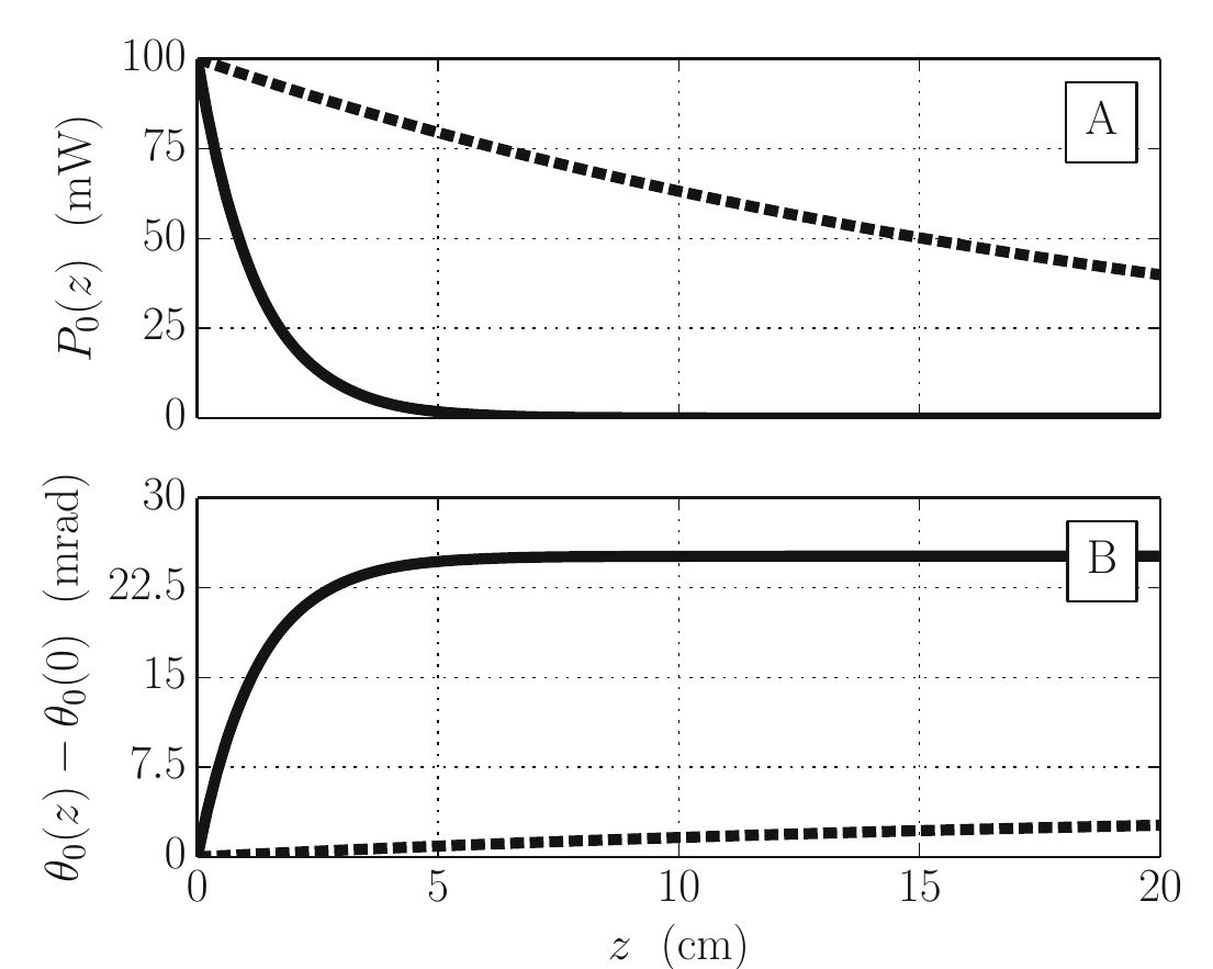
Source: P.-É. Larré et al., European Physical Journal D 71, 146 (2017). © EDP Sciences, SIF and Springer-Verlag.
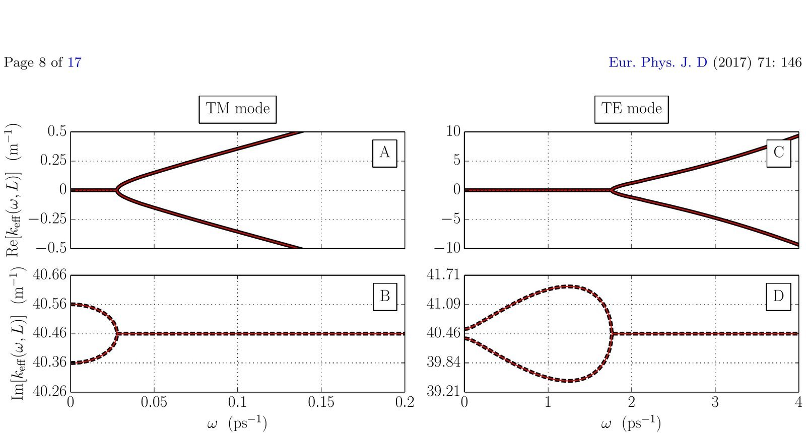
Source: P.-É. Larré et al., European Physical Journal D 71, 146 (2017). © EDP Sciences, SIF and Springer-Verlag.
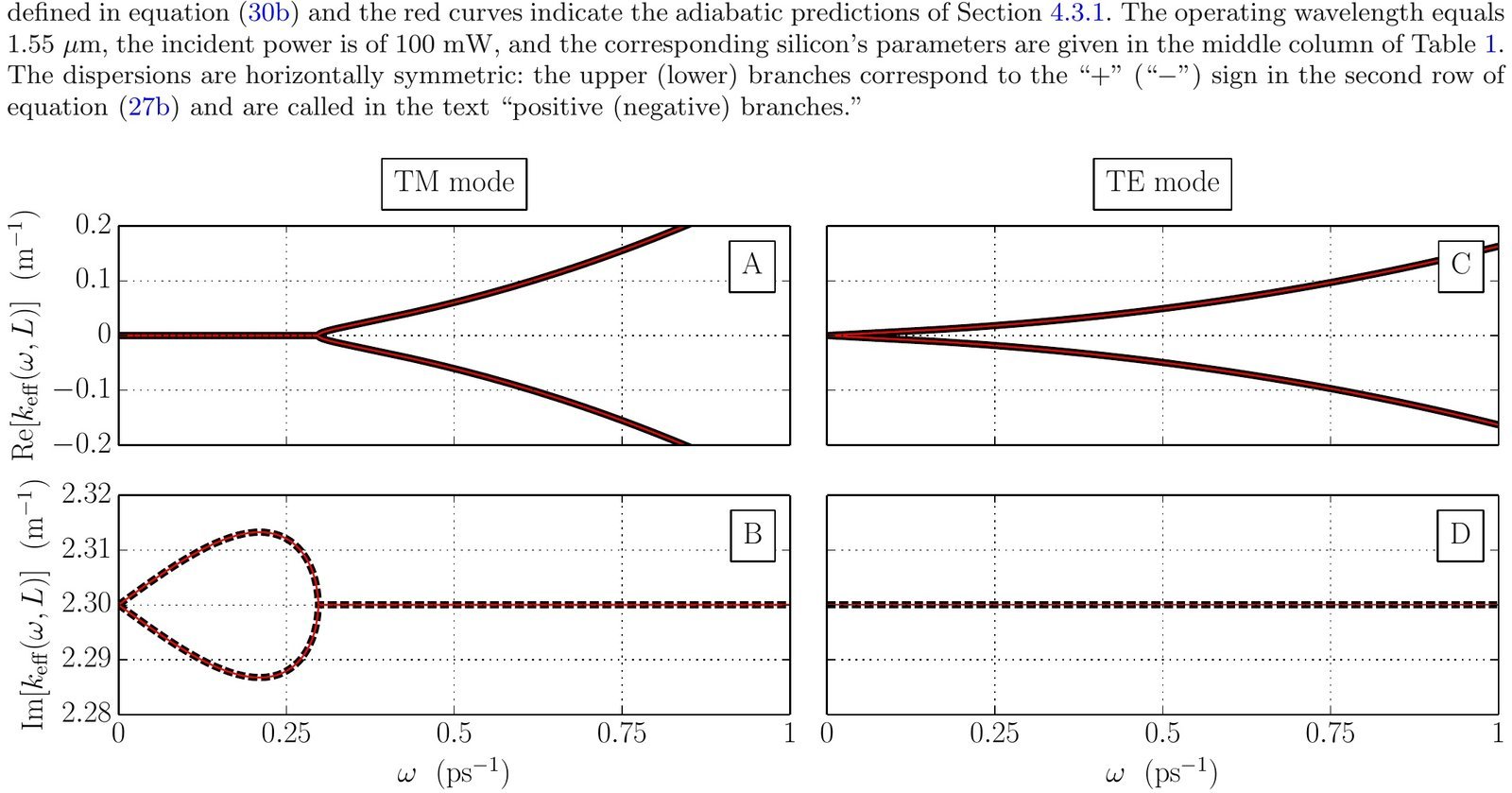
Source: P.-É. Larré et al., European Physical Journal D 71, 146 (2017). © EDP Sciences, SIF and Springer-Verlag.
Source: P.-É. Larré et al., European Physical Journal D 71, 146 (2017). © EDP Sciences, SIF and Springer-Verlag.
Source: P.-É. Larré et al., European Physical Journal D 71, 146 (2017). © EDP Sciences, SIF and Springer-Verlag.
Source: P.-É. Larré et al., European Physical Journal D 71, 146 (2017). © EDP Sciences, SIF and Springer-Verlag.
Article access and reuse
This is a subscription article. No publisher PDF is offered here; the Version of Record remains authoritative. Official Springer article record · Springer Nature rights and permissions.
Related publications

Research fields
Simulations & fits
Bogoliubov theory is adapted to weak optical fluctuations propagating on a Kerr-nonlinear pump in a single-mode channel waveguide. Analytical and numerical solutions include one- and two-photon losses and predict how a phase-sensitive stimulated four-wave-mixing measurement can reconstruct the renormalised dispersion.
Characterization
The proposed pump-probe interferometric protocol treats phase delay, not intensity alone, as the observable. This provides an experimentally accessible route to distinguish phonon-like and free-particle branches of the optical-fluid dispersion in an integrated waveguide.
RESEARCH TOPICS
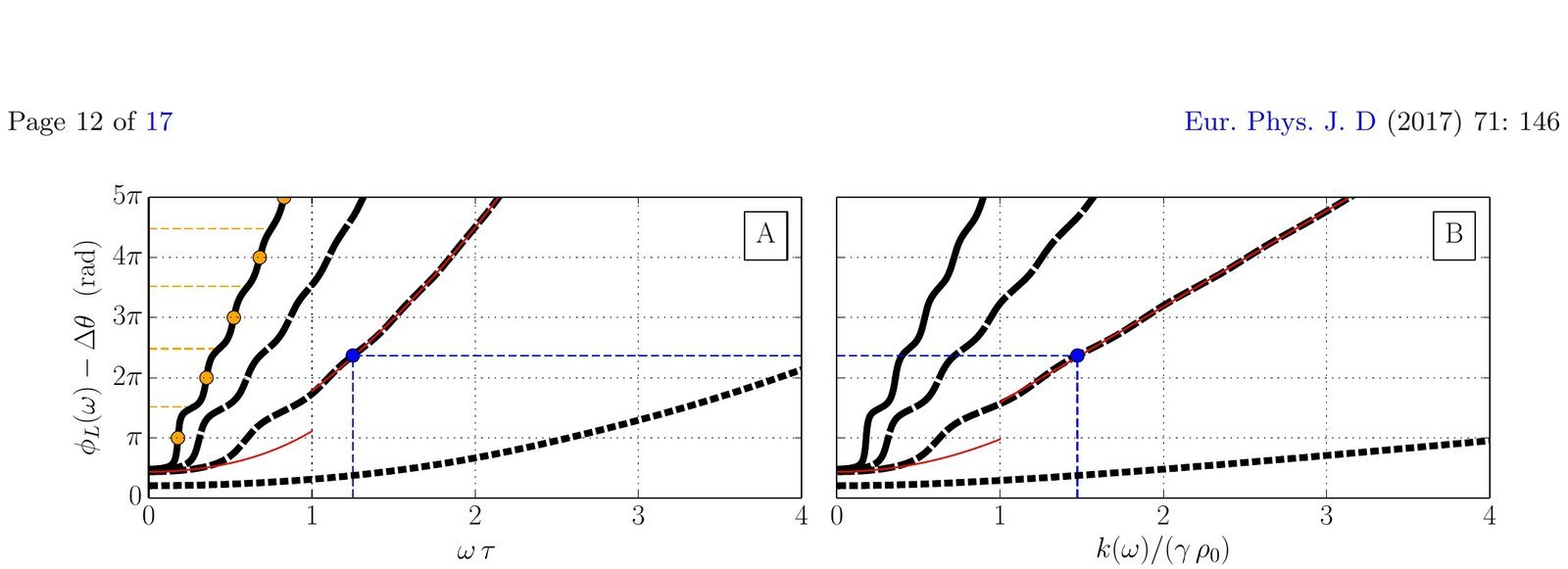
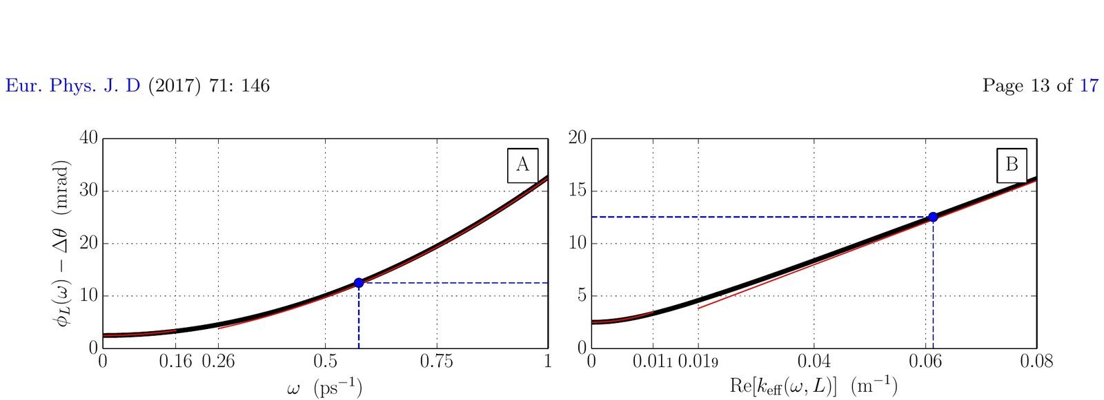
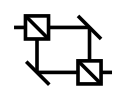 InterferenceA strong pump establishes the optical-fluid background inside a nonlinear waveguide, while a weak frequency-shifted probe accumulates a phase delay relative to a reference arm. Figures 5 and 6 show how that measured phase is related to the real part of the effective Bogoliubov wave vector.
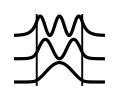 MultimodeAlthough the physical waveguide is single-mode, the linearised fluctuations have two coupled Bogoliubov components, conventionally written u and v, which mix positive- and negative-frequency perturbations around the pump. In this context “multimode” refers to the coupled excitation branches of the nonlinear optical field, not to uncontrolled transverse waveguide modes.
 NonlinearKerr refraction supplies the effective photon-photon interaction that gives the optical beam its fluid-like collective dispersion. The paper therefore tests how far the conservative Bogoliubov picture survives in a driven, absorbing nonlinear waveguide.
 QuantumBogoliubov theory, originally developed for weak excitations of a Bose quantum fluid, is applied to fluctuations riding on a coherent optical pump. The predicted dispersion contains a sound-like collective regime but is modified by propagation and two-photon losses.
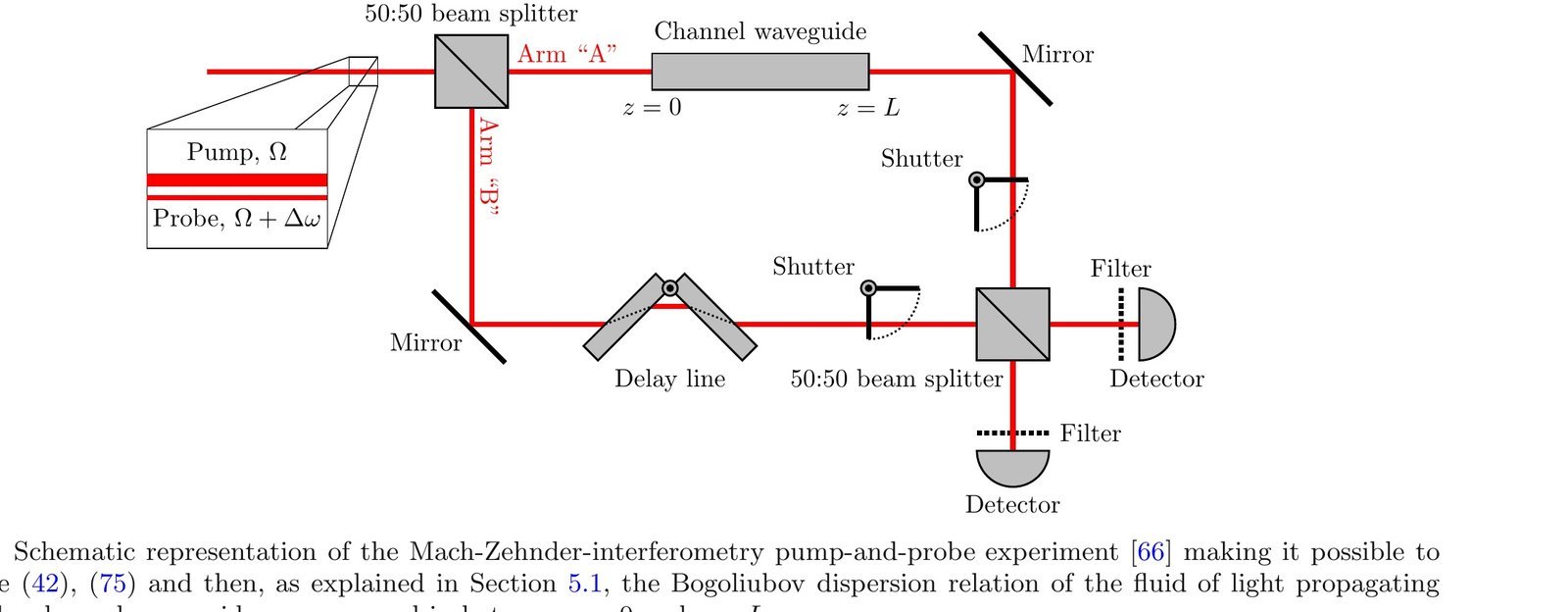
 SetupsThe experimental proposal sends pump and probe through the nonlinear waveguide in one Mach-Zehnder arm while the other arm supplies a phase reference. The chosen geometry turns a theoretical dispersion relation into an observable quantity and explicitly accounts for the finite 2 cm propagation length, coupling losses and polarization-dependent silicon parameters.